Using Google Spreadsheet to Track a Stock Portfolio
I use a Google Sheet to track my stock portfolio. This is an example of what the spreadsheet looks like. If you just want to download a copy scroll to the bottom of this page.
I chose Google Sheets because it can query Google Finance to pull market data. This helps me identify which stocks in my portfolio are reaching a trigger point where I may want to buy, which I typically base on P/E ratio.
Google Finance functions
First, let’s cover what financial data Google Sheets can pull in. According to the help page, the GoogleFinance function will let us pull in these attributes for an equity:
- price: market price of the stock – delayed by up to 20 minutes.
- priceopen: the opening price of the stock for the current day.
- high: the highest price the stock traded for the current day.
- low: the lowest price the stock traded for the current day.
- volume: number of shares traded of this stock for the current day.
- marketcap: the market cap of the stock.
- tradetime: the last time the stock traded.
- datadelay: the delay in the data presented for this stock using the googleFinance() function.
- volumeavg: the average volume for this stock.
- pe: the Price-to-Earnings ratio for this stock.
- eps: the earnings-per-share for this stock.
- high52: the 52-week high for this stock.
- low52: the 52-week low for this stock.
- change: the change in the price of this stock since yesterday’s market close.
- beta: the beta value of this stock.
- changepct: the percentage change in the price of this stock since yesterday’s close.
- closeyest: yesterday’s closing price of this stock.
- shares: the number of shares outstanding of this stock.
- currency: the currency in which this stock is traded.
So if we want to use the GoogleFinance function to display one of these attributes we use the following formula in the spreadsheet cell:
=GoogleFinance("symbol"; "attribute")
For example, if we want to display the current P/E ratio for Apple, we use this formula in the spreadsheet cell:
=GoogleFinance("AAPL"; "pe")
Easy enough, right?
The spreadsheet in detail
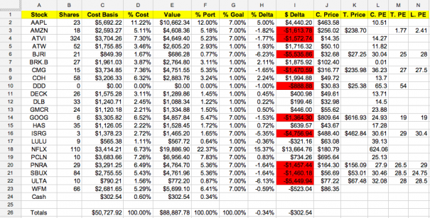
![]()
Across the top of the spreadsheet there are 14 column headers. Let’s run through these one-by-one.
Column A – Stock
We enter the symbol of the stocks we either own or are looking to add in this column.
Column B – Shares
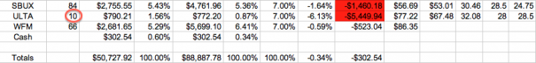
The number of shares we currently own of the stock. If it’s a stock we don’t own yet, we enter a zero.
Column C – Cost basis
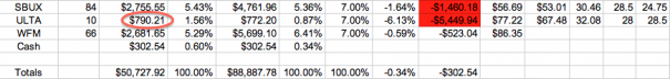
The cost basis of the shares we own. After I purchase a new position or I sell shares, I update this cell with the cost basis provided to me in my brokerage account.
Column D – % Cost
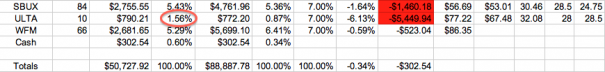
The cost basis of the position represented as a percentage of the whole portfolio, automatically calculated.
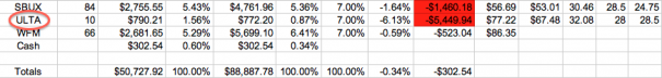
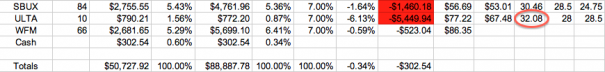
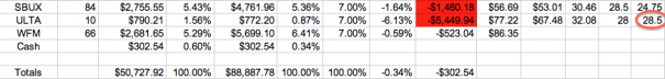
In this example, it is the $790.21 cost basis of ULTA divided by the $50,727.92 total cost basis of the portfolio. This helps me gauge if the stock is doing the heavy lifting or if I am by adding cash to the position.
Column E – Value
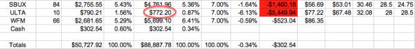
The real time value of the position. In this example, the number of ULTA shares in Column B, 10, is multiplied by the real time share price in Column J, $77.22.
Column F – % Port
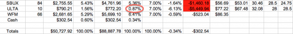
This value is the percentage the position represents as part of the portfolio. In this example, the value of the position in Column E, $772.20, is divided by the $88,887.78 total value of the portfolio.
Column G – % Goal
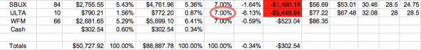
This is the percentage of the portfolio we want to target for the position. I personally set targets at 0.5%, 1%, 3%, 5%, and 7%.
Column H – % Delta
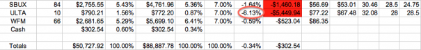
The percentage we want the position to be less the current percentage of the position determines the percentage delta.
In this example, we want ULTA to be 7.00% of our portfolio (the target goal in Column G) and subtract the current percentage of the position in Column F, 0.87%.
This value is automatically calculated and will fluctuate based on the whole portfolio.
Column I – $ Delta
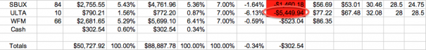
Based on the percentage of our portfolio we want to allocate towards the stock, this is the real time dollar amount our position is overweight/underweight.
It’s automatically calculated by taking the delta percentage in Column H (in this example -6.13%) multiplied by the $88,887.78 total value of the portfolio. Therefore, if we want a full position in ULTA right now, we need to purchase an additional $5,449.94 worth of shares.
I like to highlight the spreadsheet cells in red whenever this dollar amount exceeds a threshold in order to highlight positions where cash needs to be added.
Column J – Current price
The current share price, which can be delayed by up to 20 minutes. To get this data we use the ticker symbol in Column A within the cell like this:
=GoogleFinance(A22;)
Or we can use the ticker symbol directly in the cell like this:
=GoogleFinance("ULTA")
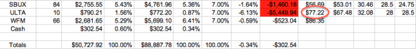
Column K – Target price
The real-time share price we’re targeting to add shares. For most of my stocks this is usually based on the P/E ratio so the function in this cell is:
=GoogleFinance("ULTA"; "EPS") * M22
This tells Google Finance to query the current EPS of ULTA and then the spreadsheet takes that value, multiplies it by my target P/E of 28 in Column M, and then displays the share price where I should target shares.
I also find it useful to have the current price in a column next to the target price, so we can do a quick scan to know where the prices are coming inline.
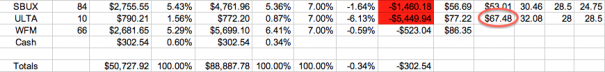
Column L – Current P/E
The current P/E ratio. The ticker symbol in Column A can be used in the cell like this:
=GoogleFinance(A22;"pe")
Or we can use the ticker symbol directly in the cell like this:
=GoogleFinance("ULTA";"pe")
Column M – Target P/E
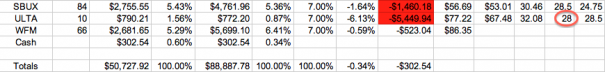
We need to fill this cell in with the target P/E where we want to add more shares. In this example I am targeting a P/E of 28 to add more shares of ULTA.
This value is used in Column K to calculate the accompanying share price. I also find it useful to have the current P/E in a column next to the target P/E, so we can do a quick scan to know when the P/E values are coming inline.
Column N – Last P/E
Completely optional, but I use this column to track the P/E when I last purchased shares. One of my goals is to add shares at better value points (a lower multiple), so it’s a quick reference.
Maintenance and mistake proofing
The only maintenance required for the spreadsheet is to:
- Update the cost basis and number of shares when positions are bought or sold.
- Update the Cash value in Column A when new cash is added to the portfolio, or when positions are bought and sold.
The totals across the bottom of the spreadsheet ensure there are no mistakes in the spreadsheet.